I am new to quantitative finance, and I wanted to start with something foundational but still mathematical. Portfolio optimization felt like the right first topic. I had heard the phrase many times, but I did not really know what the first principles looked like.
That led me to Markowitz’s 1952 paper, Portfolio Selection. I expected a short historical paper. What I found was a surprisingly visual argument: in the three-security case, return becomes a family of straight lines, variance becomes a family of ellipses, and the feasible portfolios sit inside a triangle.
This post is my worked reading note. I am not trying to write a finance textbook. I am trying to record how the geometry made the usual diversification story feel concrete.
Markowitz separates portfolio selection into two stages. First, we form beliefs about the securities: their expected returns, their variances, and how they move together. Then we use those beliefs to choose portfolio weights. The paper mostly studies the second stage. It asks: if we already have expected returns and covariances, how should we choose the portfolio?
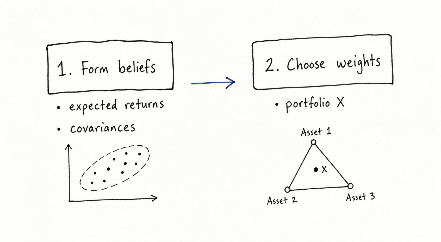
AI-generated handwritten-style sketch, created with GPT-Image-2 for this post. It is my visual summary of the two-stage setup, not a figure from Markowitz.
I use Markowitz-style notation below. Suppose there are $n$ securities, and let $i$ index one of them. The anticipated return of security $i$ is $R_i$, and the portfolio weight in that security is $X_i$, meaning the fraction of wealth invested there. I write the return vector as $R=(R_1,\ldots,R_n)^\top$ and the weight vector as $X=(X_1,\ldots,X_n)^\top$. The covariance matrix is $\Sigma$; its diagonal entries are variances, and its off-diagonal entries are covariances. I use $E$ for portfolio expected return and $V$ for portfolio variance. In this post, variance is the mathematical version of risk.
The main question is: which weights $X$ are worth considering once we care about both return and risk?
Why return alone is not enough
The tempting first rule is simple: choose the portfolio with the largest anticipated return. This is the rule Markowitz pushes against. If the portfolio return is called $R_p$, then
\[R_p=\sum_i X_iR_i.\]For now, I am assuming the same simple constraint used in the geometric examples: no short selling and all wealth invested. That is,
\[\sum_i X_i=1,\qquad X_i\ge 0,\]This means $R_p$ is only a weighted average. If the best individual anticipated return is $R_m=\max_i R_i$, then every $R_i\le R_m$, so
\[R_p=\sum_i X_iR_i\le \sum_i X_iR_m=R_m.\]This is the problem. A return-only rule either puts everything into the single highest-return security, or it is indifferent among securities tied for highest return. There is no place in the rule where diversification can enter.
Markowitz’s replacement is to consider return and variance together:
\[E=R^\top X,\qquad V=X^\top\Sigma X.\]Here $R^\top X$ is the same weighted-average return as above, just written in vector notation. The variance formula $X^\top\Sigma X$ is different. It contains all pairwise covariance terms through $\Sigma$.
This is the asymmetry I want to keep in view: expected return is linear in the weights, while variance is quadratic in the weights. That quadratic term is where diversification enters the math. If assets do not move perfectly together, a mixture can reduce variance without giving up return in the same proportion. A return-only rule cannot see this. A mean-variance rule can.
What does efficient mean?
Once return and variance are both in the picture, I cannot just ask for “the best” portfolio without saying what best means. Of course I would like more expected return. Of course I would like less variance. But these two wishes can point in different directions.
Some comparisons are still easy. If one portfolio gives the same return with lower variance, I would rather hold that one. If it gives higher return with the same variance, I would rather hold that one too. The hard cases are the tradeoffs: higher return and higher variance, or lower variance and lower return. At that point the math has not chosen for us. We need a risk preference.
Say portfolio $X$ has return and variance
\[(E_X,V_X),\]and another feasible portfolio $Y$ has
\[(E_Y,V_Y).\]Portfolio $Y$ dominates portfolio $X$ if
\[E_Y\ge E_X,\qquad V_Y\le V_X,\]and at least one of those two inequalities is strict. In words, $Y$ is at least as good on both dimensions and strictly better on one. It gives no less return with no more variance, or the same variance with more return.
A portfolio is efficient if no feasible portfolio dominates it. Equivalently, $X$ is efficient if there is no other feasible $Y$ such that
\[E_Y\ge E_X,\qquad V_Y\le V_X,\]with at least one strict improvement.
This definition is why the efficient set is usually a frontier rather than a single point. Along the frontier, moving toward higher return usually means accepting higher variance. Moving toward lower variance usually means accepting lower return. Markowitz gives us the set of reasonable candidates; choosing one final portfolio still requires one more choice, such as a risk-aversion parameter, a target return, or a maximum acceptable variance.
Here is a tiny example.
| Portfolio | Expected return | Variance |
|---|---|---|
| A | 10% | 0.09 |
| B | 8% | 0.04 |
| C | 10% | 0.04 |
Portfolio C dominates portfolio A because it has the same return and lower variance. C also dominates B because it has the same variance and higher return. But A and B are not directly comparable: A has higher return, while B has lower variance. A reader who wants return may prefer A; a reader who hates risk may prefer B. This is why Markowitz does not simply produce one universally best portfolio without saying anything about risk preference.
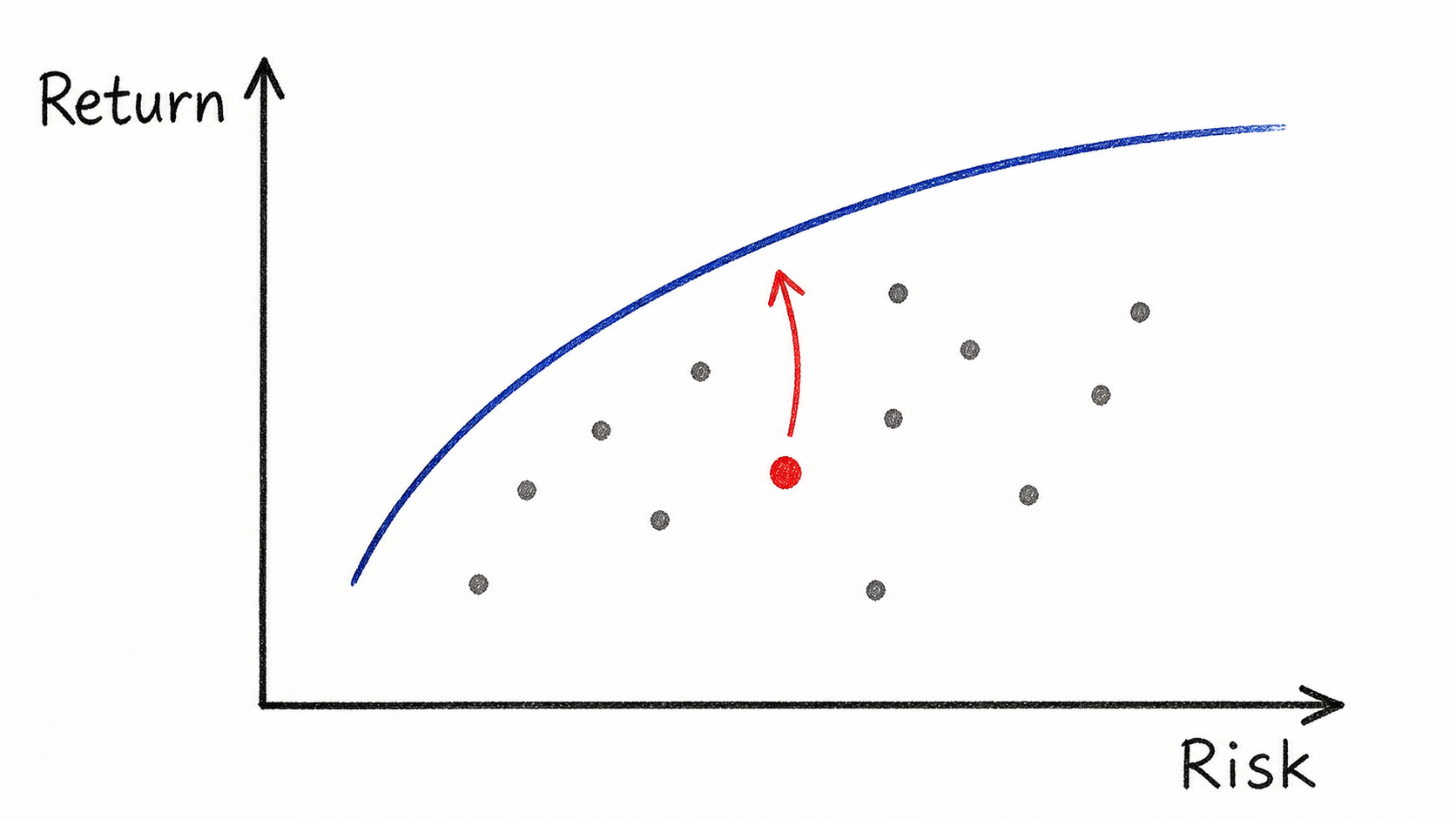
AI-generated illustration, created with GPT-Image-2 for this post. The blue curve represents nondominated portfolios. The red point is dominated because moving upward improves return at the same risk, while moving left would reduce risk at the same return.
Three securities reduce to a triangle
Now we can specialize to the picture in the paper. Markowitz’s figures use three securities. That is a convenient case because three portfolio weights can be drawn on a two-dimensional page.
There are three weights, $X_1$, $X_2$, and $X_3$. The budget constraint says
\[X_1+X_2+X_3=1,\]so once $X_1$ and $X_2$ are chosen, $X_3$ is already determined:
\[X_3=1-X_1-X_2.\]The attainable set is the triangle
\[X_1\ge 0,\qquad X_2\ge 0,\qquad X_1+X_2\le 1.\]This is the triangle that appears in the plots. The corners are the three all-in portfolios: all security 1, all security 2, or all security 3.
Expected return becomes a line in this two-dimensional picture:
\[\begin{aligned} E &=X_1R_1+X_2R_2+X_3R_3 \\ &=R_3+X_1(R_1-R_3)+X_2(R_2-R_3). \end{aligned}\]Therefore fixed-$E$ curves are straight lines in the $(X_1,X_2)$ plane. Markowitz calls these isomean lines: “iso” means same, and “mean” here means expected return. The return vector $R$ controls their slope. If we change $R$, the blue dashed lines in the widget below rotate, while the variance ellipses stay the same.
Variance becomes an ellipse
The next bit is just bookkeeping. I want to write the three weights using only the two coordinates that appear on the page.
Use
\[z=\begin{bmatrix}X_1\\X_2\end{bmatrix},\qquad e_3=\begin{bmatrix}0\\0\\1\end{bmatrix},\qquad B=\begin{bmatrix} 1&0\\ 0&1\\ -1&-1 \end{bmatrix}.\]Here $z$ is the two-dimensional coordinate in the plot. The vector $e_3$ represents the all-security-3 portfolio $(0,0,1)^\top$. The matrix $B$ tells us how the full weight vector changes when we move in the $X_1$ or $X_2$ direction.
Then the full three-security weight vector can be written as
\[X=e_3+Bz = \begin{bmatrix} X_1\\ X_2\\ 1-X_1-X_2 \end{bmatrix}.\]Now substitute this into variance. This is where the ellipses come from:
\[\begin{aligned} V &=(e_3+Bz)^\top\Sigma(e_3+Bz)\\ &=z^\top B^\top\Sigma Bz +2(B^\top\Sigma e_3)^\top z +e_3^\top\Sigma e_3. \end{aligned}\]To keep the expression readable, define
\[A=B^\top\Sigma B,\qquad b=B^\top\Sigma e_3,\qquad c=e_3^\top\Sigma e_3.\]Here $A$ is a $2\times 2$ matrix, $b$ is a two-dimensional vector, and $c$ is a scalar.
Then
\[V(z)=z^\top A z+2b^\top z+c.\]This is a two-dimensional quadratic function. A level curve means “all points with the same value of $V$.” The reason those level curves are ellipses is the same reason a simple equation like
\[ax^2+by^2=k,\qquad a>0,\;b>0\]draws an ellipse: the squared terms measure distance from a center, but the two directions may be stretched by different amounts.
In the general case, the expression has a cross term and a linear term, so the ellipse may be tilted and shifted. The center of the ellipses is the point where the unconstrained variance is smallest. I call that point $z_0$. Complete the square around it:
\[V(z) = (z-z_0)^\top A(z-z_0) + \text{constant}.\]If $A$ is positive definite, the quadratic form is bowl-shaped rather than saddle-shaped. In that case, the eigenvectors of $A$ give the principal axes of the ellipse, and the eigenvalues control how quickly variance increases along those axes. A larger eigenvalue means variance rises faster in that direction, so the ellipse is narrower there. This is what the black curves in the plots show: all points on the same black curve have the same variance.
The unconstrained minimum-variance point, which is also the center of the ellipses, solves
\[\nabla V=2Az+2b=0,\]so
\[z_0=-A^{-1}b.\]If $z_0$ lies inside the triangle, the minimum-variance feasible portfolio is an interior point. If $z_0$ lies outside the triangle, the investor cannot hold that unconstrained minimum-variance portfolio under the long-only constraint. The best feasible low-variance portfolio must then occur on the boundary of the triangle.
Critical line
The critical line is the part of the figure that took me the longest to internalize. It is not an extra constraint. It is the unconstrained path of tangency points between the isomean lines and the isovariance ellipses. Isovariance just means “same variance,” so these are the black ellipse level curves from the previous section.
The sketch below is the picture I wish I had drawn earlier. The blue lines are equal-return lines. The black ellipses are equal-variance curves. The red dots are the points where a return line just touches a variance ellipse, and the red dashed path through those dots is the critical line.
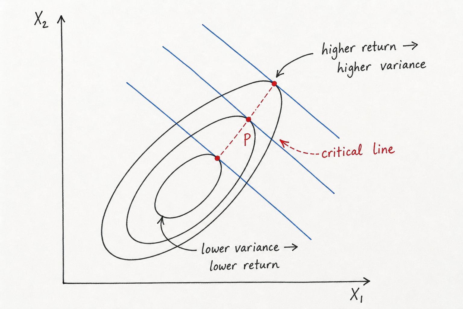
AI-generated handwritten-style sketch, created for this post. The blue lines are fixed-return lines, the black ellipses are fixed-variance curves, and the red dots are the tangency points that form the critical line.
This is why the critical-line points are efficient in the unconstrained picture. If I start at the middle red point and ask for a higher return, I have to move to a higher blue line. The tangency point on that higher blue line sits on a larger ellipse, so the variance is higher. If instead I ask for lower variance, I have to move inward to a smaller ellipse. The tangency point there lies on a lower blue line, so the return is lower. Around the critical line, return and variance are trading off against each other rather than one point simply beating another.
The calculation behind that picture is short. Fix a target expected return $E^\star$. Among all points on that fixed-return line, we want the point with the smallest variance. Geometrically, that is where the fixed-return line first touches a variance ellipse. If the line cuts through an ellipse, then there are nearby points on the same return line with smaller variance. At the minimum-variance point for that return level, the return line is tangent to the variance ellipse.
In calculus terms, minimizing $V$ while holding $E$ fixed gives the condition
\[\nabla V = \lambda \nabla E\]for some multiplier $\lambda$. This says the two gradients are parallel, which is the same as saying the two level curves are tangent.
The gradient of expected return in the $(X_1,X_2)$ plane is
\[\nabla E= \begin{bmatrix} R_1-R_3\\ R_2-R_3 \end{bmatrix}.\]The tangency direction solves
\[Ad=\nabla E,\]so
\[d=A^{-1}\nabla E,\qquad z(t)=z_0+td.\]Here $d$ is a direction vector, and $t$ is just a scalar parameter that moves us along the line. Before imposing the long-only triangle, this is the direction along which the minimum-variance point moves as we ask for higher expected return. In that unconstrained picture, the relevant part of the critical line is efficient: for each return level, the tangency point is the lowest-variance way to get that return.
The triangle constraint changes the story. The line may pass through the feasible triangle, hit a boundary, or miss the triangle completely. When it is inside the triangle and moving in the direction of increasing return from the minimum-variance point, it traces the interior part of the efficient frontier. Once it leaves the triangle, the efficient set continues along a boundary if no interior point can dominate it.
To check whether the critical line intersects the attainable triangle, solve the three inequalities:
\[z_1(t)\ge 0,\qquad z_2(t)\ge 0,\qquad z_1(t)+z_2(t)\le 1.\]Each inequality gives an interval of allowed $t$. The critical line intersects the triangle exactly when the three intervals overlap.
Efficient frontier as optimization, not a grid cloud
One implementation detail is worth making explicit. It is tempting to draw a grid of many portfolios and keep the nondominated dots. That is useful for intuition, but it is not the mathematical frontier.
For a fixed target return $E^\star$, the efficient candidate is the solution of
\[\min_X\quad X^\top\Sigma X\]subject to
\[\mathbf{1}^\top X=1,\qquad R^\top X=E^\star,\qquad X_i\ge 0.\]Here $\mathbf{1}$ is the vector of all ones, so $\mathbf{1}^\top X=1$ is the same budget constraint as before.
Sweeping $E^\star$ from the global minimum-variance return to the maximum attainable return produces a thin efficient curve.
This distinction matters. A grid-based Pareto filter can create a dense cloud near tangencies, because many nearby grid points are almost nondominated numerically. The target-return optimization gives the cleaner object: for each required return, keep the lowest-variance portfolio that can achieve it.
How the five notebook cases were designed
After working through the paper figures, I rebuilt five cases in the notebook. The knobs are exactly the two objects from the notation section:
- $R$, which rotates the isomean lines.
- $\Sigma$, which moves the ellipse center $z_0$ and changes the ellipse shape.
When reading the plots, it helps to keep four objects separate:
- The triangle is the set of portfolios we are allowed to hold.
- The blue dashed lines are equal-return lines. Moving to a higher blue line means higher $E$.
- The black ellipses are equal-variance curves. Moving toward the ellipse center means lower $V$.
- The red curve is the efficient set: the portfolios that survive the dominance test.
The efficient set is not simply “the top of the triangle” or “the closest point to the ellipse center.” It is where the two goals meet: among portfolios that can achieve a given return, it keeps the lowest-variance ones.
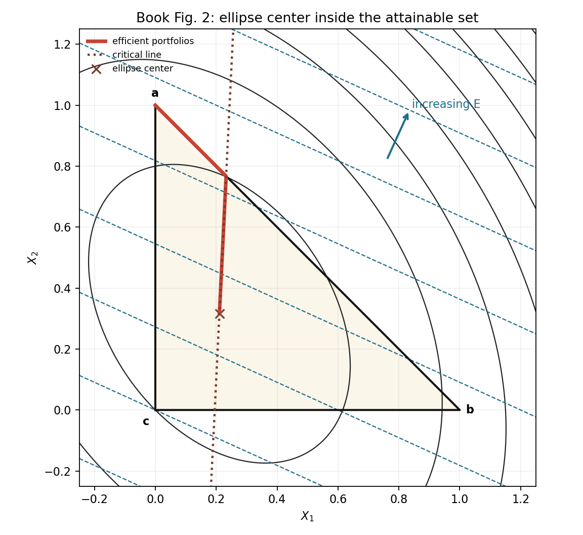
Book Fig. 2: center inside the attainable triangle
This is the cleanest case. We choose $\Sigma$ so the ellipse center $z_0$ is inside the triangle. The efficient set starts near the interior low-variance point and then moves toward higher-return portfolios.
The inputs are
\[R=\begin{bmatrix}0.08&0.14&0.03\end{bmatrix}, \qquad \Sigma= \begin{bmatrix} 0.09&0&0\\ 0&0.06&0\\ 0&0&0.04 \end{bmatrix}.\]Using $X_3=1-X_1-X_2$, the expected return becomes
\[E=X_1R_1+X_2R_2+(1-X_1-X_2)R_3 =0.03+0.05X_1+0.11X_2.\]So the isomean lines have normal vector
\[\nabla E= \begin{bmatrix} R_1-R_3\\ R_2-R_3 \end{bmatrix} = \begin{bmatrix} 0.05\\ 0.11 \end{bmatrix}.\]The variance is
\[V=X^\top\Sigma X =0.09X_1^2+0.06X_2^2+0.04(1-X_1-X_2)^2.\]After collecting terms,
\[V=0.13X_1^2+0.08X_1X_2+0.10X_2^2-0.08X_1-0.08X_2+0.04.\]In the form $V(z)=z^\top A z+2b^\top z+c$, where $z=(X_1,X_2)^\top$,
\[A= \begin{bmatrix} 0.13&0.04\\ 0.04&0.10 \end{bmatrix}, \qquad b= \begin{bmatrix} -0.04\\ -0.04 \end{bmatrix}, \qquad c=0.04.\]The ellipse center is
\[z_0=-A^{-1}b= \begin{bmatrix} 0.210526\\ 0.315789 \end{bmatrix}.\]This point is feasible because both coordinates are nonnegative and
\[0.210526+0.315789<1.\]The critical-line direction is
\[d=A^{-1}\nabla E = \begin{bmatrix} 0.052632\\ 1.078947 \end{bmatrix}, \qquad z(t)=z_0+td.\]That is why the picture shows an interior ellipse center and an efficient set that begins near the low-variance interior region before moving toward the high-return edge.
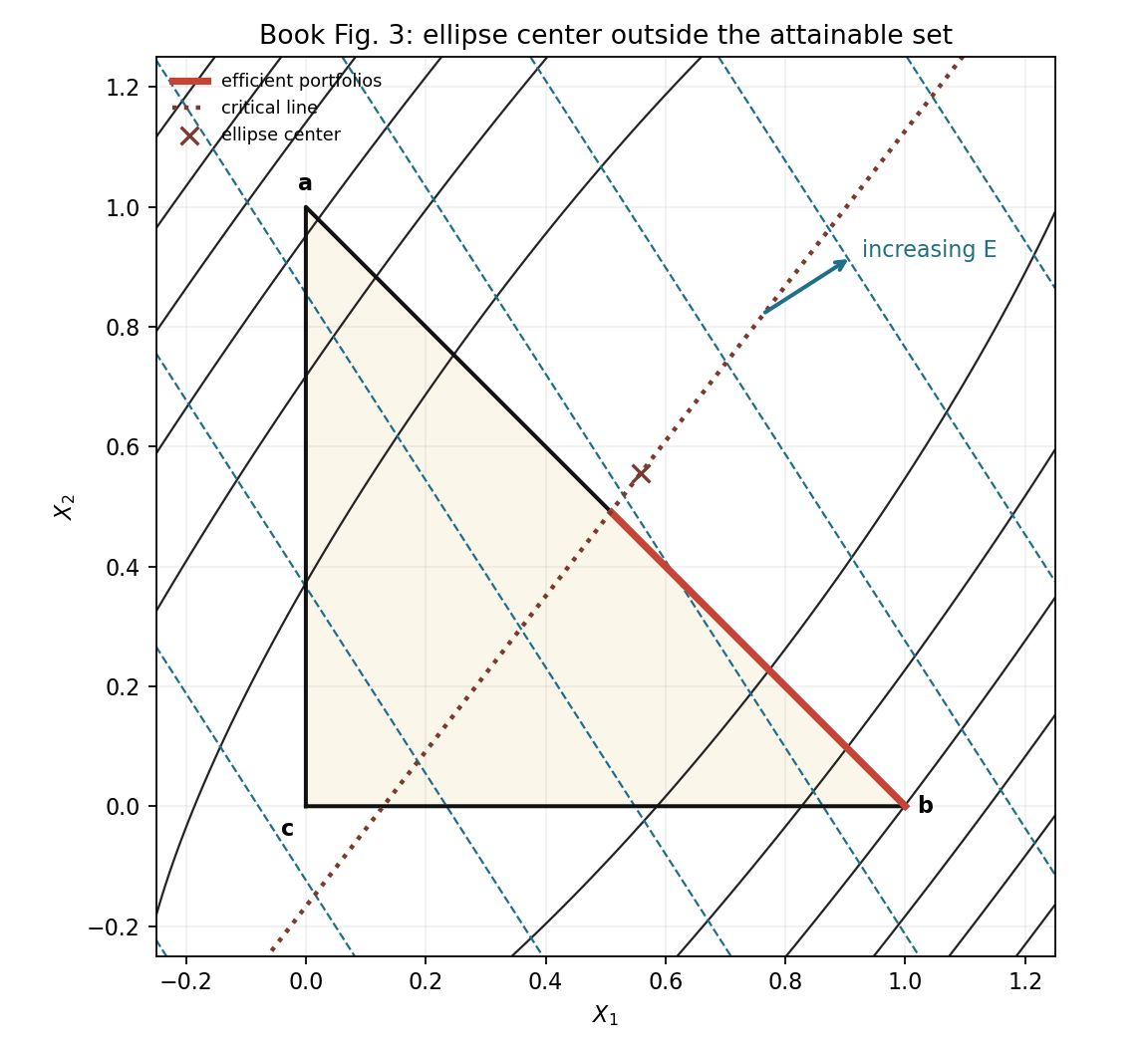
Book Fig. 3: center outside the attainable triangle
Here the unconstrained minimum-variance point is outside the triangle. The lowest reachable variance is no longer at the ellipse center itself; it is forced onto the feasible boundary.
The inputs are
\[R=\begin{bmatrix}0.143594&0.140737&0.135630\end{bmatrix}, \qquad \Sigma= \begin{bmatrix} 4.515211&-4.122941&-0.395992\\ -4.122941&4.859773&1.065369\\ -0.395992&1.065369&0.831767 \end{bmatrix}.\]The expected return plane is
\[E=0.135630+0.007964X_1+0.005107X_2,\]so
\[\nabla E= \begin{bmatrix} 0.007964\\ 0.005107 \end{bmatrix}.\]Substituting $X_3=1-X_1-X_2$ into $V=X^\top\Sigma X$ gives
\[\begin{aligned} V={}&4.515211X_1^2+4.859773X_2^2+0.831767(1-X_1-X_2)^2\\ &-8.245882X_1X_2-0.791983X_1(1-X_1-X_2) +2.130738X_2(1-X_1-X_2). \end{aligned}\]After collecting terms,
\[V=6.138961X_1^2-7.921103X_1X_2+3.560802X_2^2-2.455517X_1+0.467204X_2+0.831767.\]Therefore
\[A= \begin{bmatrix} 6.138961&-3.960551\\ -3.960551&3.560802 \end{bmatrix}, \qquad b= \begin{bmatrix} -1.227758\\ 0.233602 \end{bmatrix}, \qquad c=0.831767.\]The ellipse center is
\[z_0=-A^{-1}b= \begin{bmatrix} 0.558277\\ 0.555348 \end{bmatrix}.\]This violates the triangle constraint because
\[0.558277+0.555348>1.\]The critical-line direction is
\[d=A^{-1}\nabla E= \begin{bmatrix} 0.007870\\ 0.010188 \end{bmatrix}.\]The critical line still reaches the feasible triangle, but the minimum-variance center itself is outside. The efficient set is therefore pushed onto a boundary, and in this construction security 3 drops out along the efficient part.
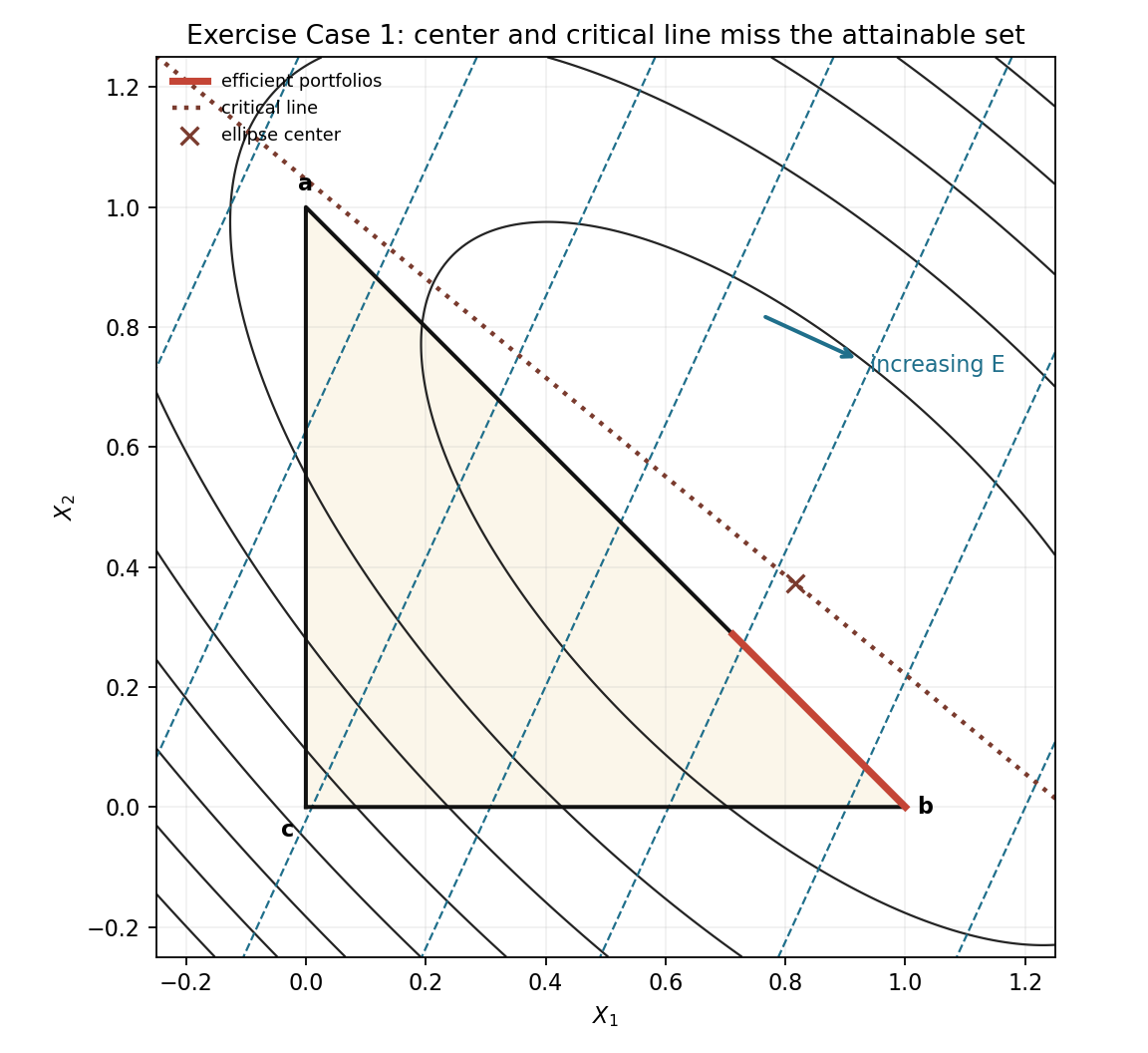
Exercise Case 1: critical line misses the triangle
This case is more extreme than Book Fig. 3. The ellipse center is outside the triangle, and the entire unconstrained critical line misses the triangle. The efficient portfolios must then live on a boundary.
The inputs are
\[R=\begin{bmatrix}0.113307&0.093703&0.099861\end{bmatrix}, \qquad \Sigma= \begin{bmatrix} 0.042838&-0.014732&0.063320\\ -0.014732&0.127790&0.095559\\ 0.063320&0.095559&0.369518 \end{bmatrix}.\]The return plane is
\[E=0.099861+0.013446X_1-0.006158X_2,\]so
\[\nabla E= \begin{bmatrix} 0.013446\\ -0.006158 \end{bmatrix}.\]The variance expands to
\[\begin{aligned} V={}&0.042838X_1^2+0.127790X_2^2+0.369518(1-X_1-X_2)^2\\ &-0.029463X_1X_2+0.126640X_1(1-X_1-X_2) +0.191117X_2(1-X_1-X_2). \end{aligned}\]After collecting terms,
\[V=0.285716X_1^2+0.391816X_1X_2+0.306191X_2^2-0.612397X_1-0.547919X_2+0.369518.\]Thus
\[A= \begin{bmatrix} 0.285716&0.195908\\ 0.195908&0.306191 \end{bmatrix}, \qquad b= \begin{bmatrix} -0.306198\\ -0.273960 \end{bmatrix}, \qquad c=0.369518.\]The ellipse center is
\[z_0= \begin{bmatrix} 0.816318\\ 0.372436 \end{bmatrix},\]which is outside the triangle because
\[0.816318+0.372436>1.\]The critical-line direction is
\[d=A^{-1}\nabla E= \begin{bmatrix} 0.108413\\ -0.089476 \end{bmatrix}.\]When we solve the three feasibility inequalities for $z(t)=z_0+td$,
\[z_1(t)\ge 0,\qquad z_2(t)\ge 0,\qquad z_1(t)+z_2(t)\le 1,\]the three intervals have no common overlap. So the unconstrained tangency path never enters the attainable triangle. The efficient set moves to the boundary $X_3=0$, which means security 3 is absent from efficient portfolios.
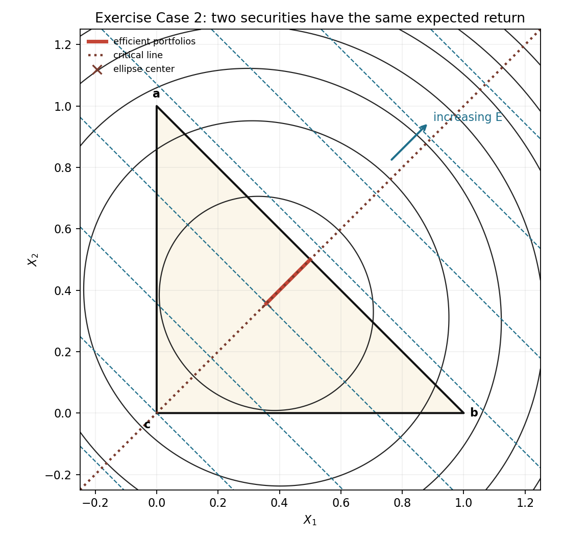
Exercise Case 2: two securities have the same expected return
This case shows why equal return does not mean equal usefulness. Securities 1 and 2 have the same expected return, but because their covariance is negative, mixing them can reduce variance.
The inputs are
\[R=\begin{bmatrix}0.12&0.12&0.05\end{bmatrix}, \qquad \Sigma= \begin{bmatrix} 0.04&-0.02&0\\ -0.02&0.04&0\\ 0&0&0.025 \end{bmatrix}.\]Since $R_1=R_2$, the return equation is
\[E=0.05+0.07X_1+0.07X_2.\]Equivalently,
\[E=0.05+0.07(X_1+X_2).\]This means return only cares about the combined weight in securities 1 and 2, not how that combined weight is split between them. Geometrically, the isomean lines are parallel to the edge joining securities 1 and 2.
The variance is
\[V=0.04X_1^2+0.04X_2^2+0.025(1-X_1-X_2)^2-0.04X_1X_2.\]After collecting terms,
\[V=0.065X_1^2+0.01X_1X_2+0.065X_2^2-0.05X_1-0.05X_2+0.025.\]So
\[A= \begin{bmatrix} 0.065&0.005\\ 0.005&0.065 \end{bmatrix}, \qquad b= \begin{bmatrix} -0.025\\ -0.025 \end{bmatrix}, \qquad c=0.025.\]The ellipse center is
\[z_0=-A^{-1}b= \begin{bmatrix} 0.357143\\ 0.357143 \end{bmatrix}.\]The critical-line direction is
\[d=A^{-1} \begin{bmatrix} 0.07\\ 0.07 \end{bmatrix} = \begin{bmatrix} 1\\ 1 \end{bmatrix}.\]The equal entries in $d$ are the main visual clue. The efficient path moves in a balanced direction between securities 1 and 2. At the high-return end, the useful portfolio is not “all security 1” or “all security 2”; it is the diversified mix that exploits their negative covariance.
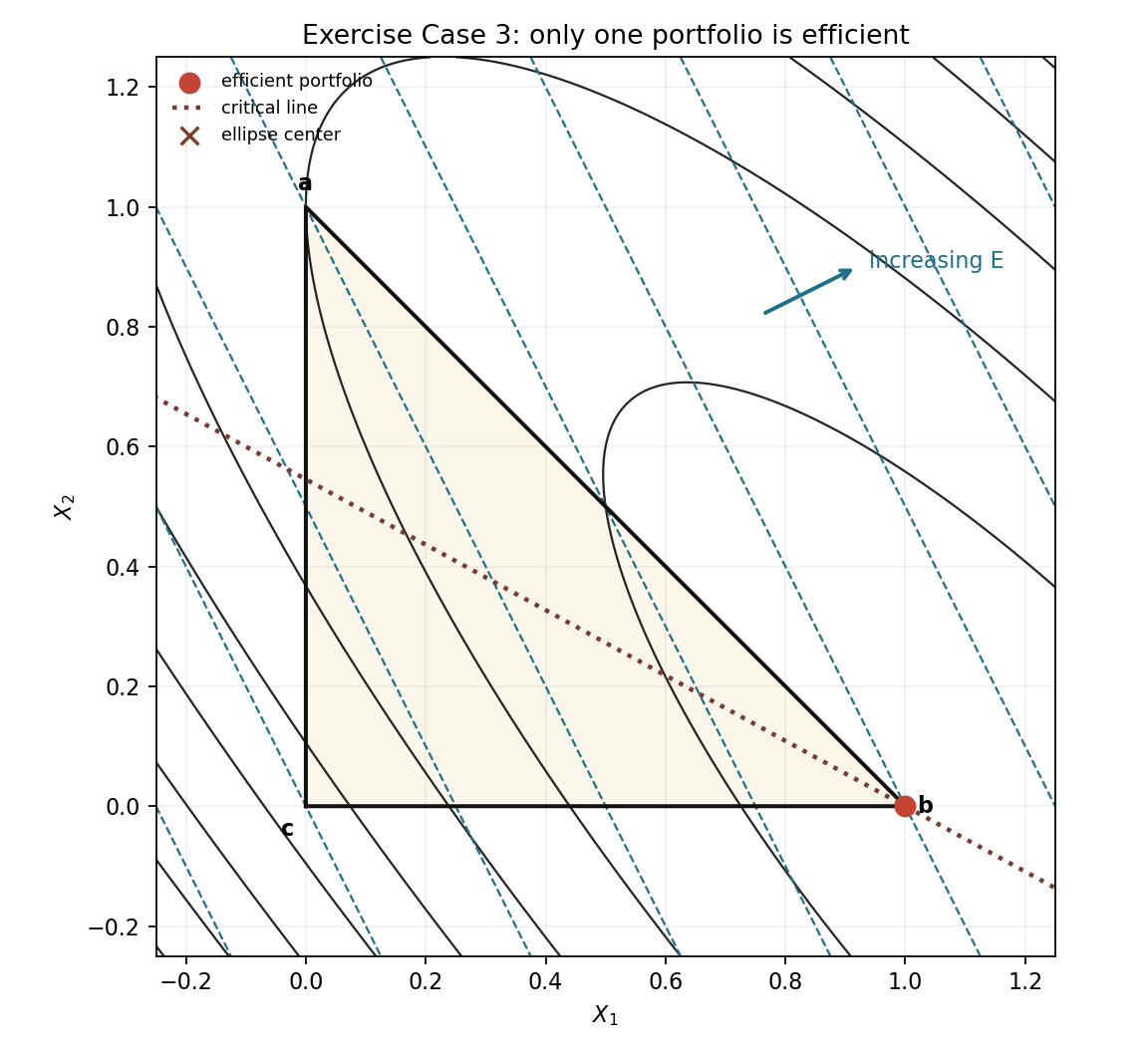
Exercise Case 3: only one portfolio is efficient
In this final case, one vertex is deliberately made both high-return and low-variance. The efficient set collapses to a single portfolio.
The inputs are
\[R=\begin{bmatrix}0.12&0.08&0.04\end{bmatrix}, \qquad \Sigma= \begin{bmatrix} 0.01&0.015&0.02\\ 0.015&0.04&0.04\\ 0.02&0.04&0.09 \end{bmatrix}.\]The expected return plane is
\[E=0.04+0.08X_1+0.04X_2.\]Security 1 has the largest return. The covariance matrix is also chosen so moving away from security 1 increases variance rather than reducing it.
The variance expands to
\[\begin{aligned} V={}&0.01X_1^2+0.04X_2^2+0.09(1-X_1-X_2)^2\\ &+0.03X_1X_2+0.04X_1(1-X_1-X_2) +0.08X_2(1-X_1-X_2). \end{aligned}\]After collecting terms,
\[V=0.06X_1^2+0.09X_1X_2+0.05X_2^2-0.14X_1-0.10X_2+0.09.\]Thus
\[A= \begin{bmatrix} 0.06&0.045\\ 0.045&0.05 \end{bmatrix}, \qquad b= \begin{bmatrix} -0.07\\ -0.05 \end{bmatrix}, \qquad c=0.09.\]The ellipse center is
\[z_0=-A^{-1}b= \begin{bmatrix} 1.282051\\ -0.153846 \end{bmatrix}.\]That center is infeasible because $X_2<0$. The critical-line direction is
\[d=A^{-1} \begin{bmatrix} 0.08\\ 0.04 \end{bmatrix} = \begin{bmatrix} 2.256410\\ -1.230769 \end{bmatrix}.\]The direction points even farther toward security 1 and away from security 2. Within the feasible triangle, the portfolio $(1,0,0)$ has the highest expected return and is not beaten on variance by any other feasible mixture. Every other point is dominated, so the efficient frontier is just that one vertex.
Interactive reconstruction
Use the preset menu to recreate the five notebook plots. Then edit $R$ or the symmetric matrix $\Sigma$ directly.
The matrix below is the covariance matrix used by the geometry. If you want to think in correlation-matrix terms, set the diagonal entries to $1$ and use correlations as the off-diagonal entries. The notebook cases use covariance matrices, so the presets keep the original $\Sigma$ values.
A good way to use the widget:
- Start with Book Fig. 2 and change only $R_2$. The blue isomean lines rotate, but the black ellipses do not.
- Change one diagonal entry of $\Sigma$, such as $\Sigma_{22}$. The ellipses reshape because the variance of that asset changed.
- Choose Exercise 1 and notice that the green critical line misses the triangle, so the efficient set lives on a boundary.
- Choose Exercise 3 and notice that the red efficient set collapses to one point.
Return vector $R$
Covariance / correlation-style matrix $\Sigma$
What about $N$ securities?
In fact, similar thoughts apply to the $N$-security case. The three-security triangle is only the easiest version to draw. With four securities, the feasible set becomes a tetrahedron. With $N$ securities, it becomes a higher-dimensional simplex. The core result is the same: efficient portfolios are connected line segments in portfolio-weight space.
Here is the proof in the notation I find easiest to remember. Suppose there are $N$ securities. A long-only portfolio is a vector $x\in\mathbb{R}^N$ satisfying
\[\mathbf{1}^\top x=1,\qquad x_i\ge 0.\]The expected return and variance are
\[E(x)=\mu^\top x,\qquad V(x)=x^\top\Sigma x,\]where $\mu$ is the vector of expected returns and $\Sigma$ is the covariance matrix. To trace the efficient set, fix a target return $e$ and ask for the minimum-variance portfolio that reaches that return:
\[\min_x\; x^\top\Sigma x\]subject to
\[\mathbf{1}^\top x=1,\qquad \mu^\top x=e,\qquad x_i\ge 0.\]The inequality $x_i\ge 0$ is handled face by face. Fix an active set $A$, meaning the securities whose weights are currently positive. On that face of the simplex, the inactive securities have weight zero and the active weights satisfy
\[\mathbf{1}_A^\top x_A=1,\qquad x_i>0\quad(i\in A).\]While the active set stays fixed, the first-order condition for the equality-constrained minimum has the form
\[2\Sigma_{AA}x_A=\alpha \mathbf{1}_A+\beta\mu_A,\]where $\alpha$ and $\beta$ are the multipliers for the budget constraint and the target-return constraint. If $\Sigma_{AA}$ is nonsingular, then
\[x_A=\frac{1}{2}\Sigma_{AA}^{-1}(\alpha\mathbf{1}_A+\beta\mu_A).\]The two numbers $\alpha$ and $\beta$ are chosen so that
\[\mathbf{1}_A^\top x_A=1,\qquad \mu_A^\top x_A=e.\]These are two linear equations whose right-hand side is $(1,e)$. Therefore $\alpha$ and $\beta$ change linearly with $e$, and so $x_A$ also changes linearly with $e$. In other words, while the active set stays fixed,
\[x_A(e)=a_A+e\,b_A\]for two fixed vectors $a_A$ and $b_A$. That is the line-segment result.
The segment is valid only while all active weights remain positive:
\[x_i(e)>0,\qquad i\in A.\]When one active weight reaches zero, the path hits a boundary face. Then that security drops out, the active set changes, and the same argument starts again on the smaller face. This is why the efficient portfolios form a chain:
\[\text{line segment}\;\to\;\text{line segment}\;\to\;\text{line segment}\;\to\cdots\]There is one last translation step. Along one segment, $x(e)=a+e b$. Expected return is already $e$, but variance becomes
\[V(e) =(a+eb)^\top\Sigma(a+eb) =a^\top\Sigma a+2e\,b^\top\Sigma a+e^2 b^\top\Sigma b.\]So a straight segment in portfolio-weight space becomes a parabola segment when plotted as variance against expected return. That is why Markowitz can say efficient portfolios are line segments, while efficient $(E,V)$ combinations are connected parabola pieces.
Convexity and mixing portfolios
Markowitz’s Figure 7 is really a convexity picture. If two portfolios have the same variance, then the straight-line mixture between them cannot move outward to a larger variance ellipse. It moves inward, or in a degenerate case stays on the same ellipse.
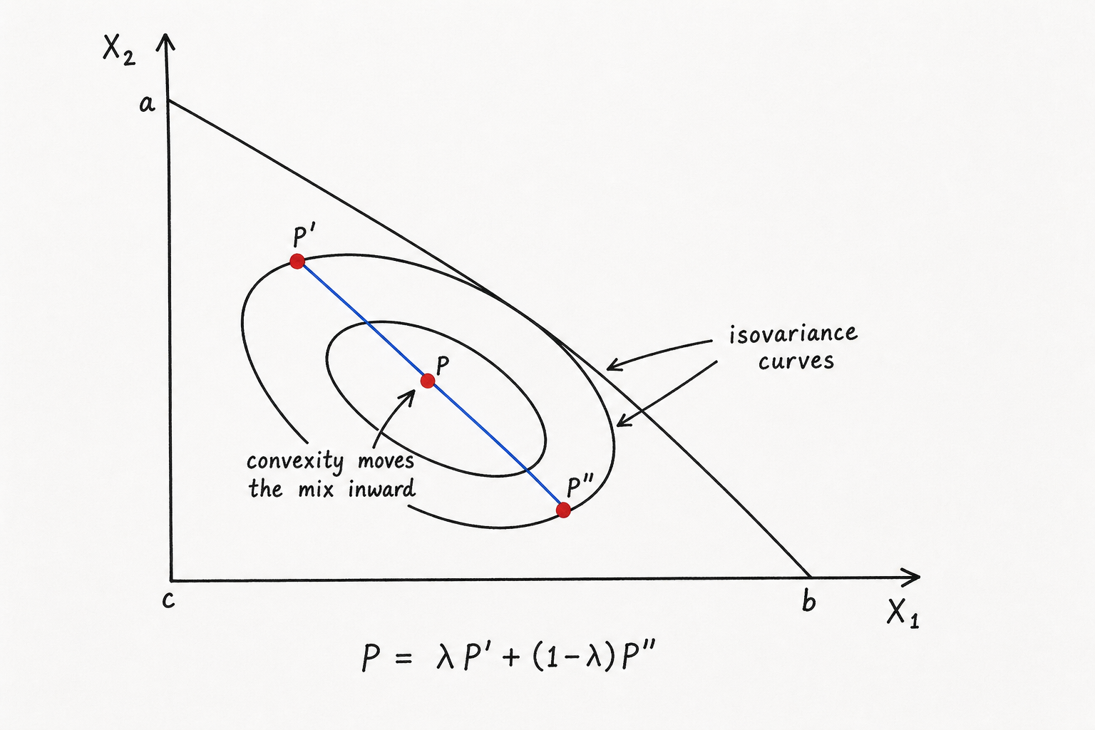
AI-generated hand-plot-style sketch, inspired by the idea in Markowitz’s Figure 7. The point $P$ is a mixture of $P’$ and $P’’$, and it falls inside a smaller isovariance curve.
Let $p$ and $q$ be two portfolios with the same variance,
\[V(p)=V(q)=v.\]For $0\le\lambda\le 1$, form the mixed portfolio
\[m_\lambda=\lambda p+(1-\lambda)q.\]Because $V(x)=x^\top\Sigma x$ is a convex quadratic form,
\[V(m_\lambda) =\lambda V(p)+(1-\lambda)V(q) -\lambda(1-\lambda)(p-q)^\top\Sigma(p-q).\]Substituting $V(p)=V(q)=v$ gives
\[V(m_\lambda) =v-\lambda(1-\lambda)(p-q)^\top\Sigma(p-q) \le v.\]That is the whole point. The lower variance is not a separate finance trick; it is the nature of convexity for the quadratic variance surface.
Takeaway
Markowitz’s main insight is not that every investor must literally use this three-security picture. The main insight is that diversification is not just a slogan. It comes from covariance.
The old rule fails because expected return alone is a weighted average. It gives no reason to diversify unless several assets tie for best expected return.
Mean-variance analysis adds the missing object: covariance. Once variance enters the decision, diversification can improve the portfolio because the covariance matrix determines whether risks offset each other.
Once we measure risk with variance, the best portfolios are no longer simply the highest-return portfolios. They are the nondominated tradeoffs between return and risk. That is the core idea behind the efficient frontier.
References and notes
- Markowitz, Harry M. “Portfolio Selection.” The Journal of Finance 7, no. 1 (1952): 77-91. DOI: 10.2307/2975974.
- Markowitz, Harry M. Portfolio Selection: Efficient Diversification of Investments. 1959. Book record available through JSTOR.
- The five geometry plots and the case-by-case algebra in this post are my own reconstruction from the accompanying Markowitz notebook. The notebook chooses each return vector $R$ and covariance matrix $\Sigma$ so the ellipse center, isomean lines, critical line, and efficient set produce the five cases shown above.
- The handwritten two-stage sketch, the critical-line sketch, the hand-plot-style dominance illustration, and the portfolio-mix convexity sketch were AI-generated for this blog post. These are explanatory visuals, not figures from Markowitz.